Notebook showing the ML-MGM method implemented in pyFRESCO

import pyfresco

Data import

In the following code cell we define the paths pointing to the img and header files of the proper hyperspectral datacube and of the summary parameters datacube. These two datacubes are the ones needed by pyFRESCO to work properly.

path_if_mtrdr = "FRT00009b5a/frt00009b5a_07_if165j_mtr3.img" # Path to the proper hyperspectral datacube
head_if_mtrdr = "FRT00009b5a/frt00009b5a_07_if165j_mtr3.hdr" # Path to the header of the proper hyperspectral datacube

path_sr_mtrdr = "FRT00009b5a/frt00009b5a_07_sr165j_mtr3.img" # Path to the summary parameters datacube
head_sr_mtrdr = "FRT00009b5a/frt00009b5a_07_sr165j_mtr3.hdr" # Path to the header of the summary parameters datacube

img , img_sr , wavelength , sr_names = pyfresco.open_raw(path_if_mtrdr , head_if_mtrdr , path_sr_mtrdr , head_sr_mtrdr) # Open the two datacubes

Nbands = len(wavelength)
print(sr_names)

['R770', 'RBR', 'BD530_2', 'SH600_2', 'SH770', 'BD640_2', 'BD860_2', 'BD920_2', 'RPEAK1', 'BDI1000VIS', 'R440', 'IRR1', 'BDI1000IR', 'OLINDEX3', 'R1330', 'BD1300', 'LCPINDEX2', 'HCPINDEX2', 'VAR', 'ISLOPE1', 'BD1400', 'BD1435', 'BD1500_2', 'ICER1_2', 'BD1750_2', 'BD1900_2', 'BD1900R2', 'BDI2000', 'BD2100_2', 'BD2165', 'BD2190', 'MIN2200', 'BD2210_2', 'D2200', 'BD2230', 'BD2250', 'MIN2250', 'BD2265', 'BD2290', 'D2300', 'BD2355', 'SINDEX2', 'ICER2_2', 'MIN2295_2480', 'MIN2345_2537', 'BD2500_2', 'BD3000', 'BD3100', 'BD3200', 'BD3400_2', 'CINDEX2', 'BD2600', 'IRR2', 'IRR3', 'R530', 'R600', 'R1080', 'R1506', 'R2529', 'R3920']

Input spectrum

The ML-MGM method is applied to a normalized spectrum. Here we reproduce a compact extraction and normalization workflow to create a target spectrum.

SE = pyfresco.SpectraExtract(img , Nbands , wavelength , 750 , 2600) # Definition of the object for spectral extraction

RGB = SE.upload_map('MAF' , folder = 'FRT00009b5a/') # Upload an RGB map for the ROI selection

target_spectra , L_target , target_mask = SE.polygon_spectra(save_pixel = True ,
 folder = 'FRT00009b5a' ,
 name = 'mgm_target_coordinates') # Select the target ROI

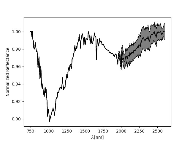
target_spectrum , target_error = SE.final_spectra(mean = True , c = 'blue') # Target mean spectrum

SN = pyfresco.SpectraNorm(RGB , Nbands , img , img_sr , wavelength ,
                         target_spectrum , target_error , target_spectra ,
                         750 , 2600)

neutral_spectra , neutral_spectrum , hull_error = SN.neutral_convex_hull() # Select the neutral ROI

norm_mgm , error_mgm = SN.norm_spectra(convex_hull=True) # Normalized spectrum
SN.normplot()

Number of points inside the drewn polygon:  425
64.25992779783394 % of the errors, set to zero for simplicity, are in reality NaN values.

The output of the above cell should look like this: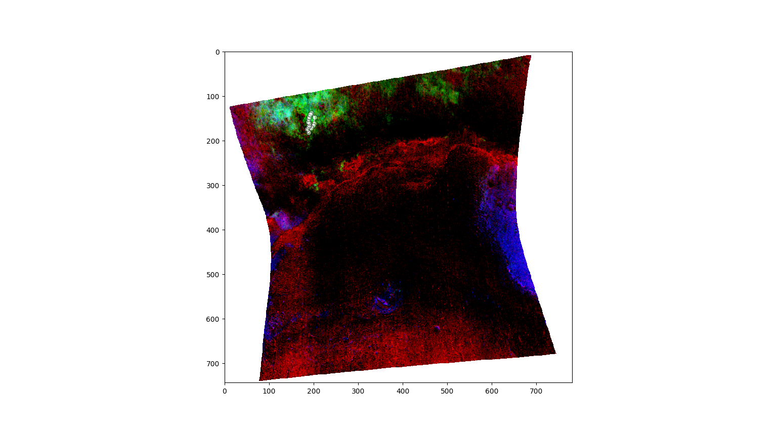

Definition of the SpectraAnalysis object

The MGM routine is part of the SpectraAnalysis class. The object is initialized with the normalized spectrum and with the spectra used to obtain it.

SA = pyfresco.SpectraAnalysis(norm_mgm , error_mgm ,
 m_spec = target_spectrum , err_spec = target_error ,
 n_spectra = neutral_spectrum , n_err = neutral_error ,
 wavelength = wavelength ,
 MIN = 750 , MAX = 2600 ,
 folder = None) # Definition of the object for spectral analysis

ML-MGM with fixed band centers

If the approximate absorption positions or their bounds are known, they can be called as parameters.

losses , gaussian_sums , n_wav , gaussian_sum , a , m , fwhm , alpha = SA.mgm(
                                                                         n = 3 ,
                                                                         iterations = 25000 ,
                                                                         lr = 0.001 ,
                                                                         means = None,
                                                                         mean_ranges = None,
                                                                         asym = True ,
                                                                         smooth = True ,
                                                                         hull = True ,
                                                                         t = 'savgol' ,
                                                                         w = 7 ,
                                                                         o = 2) # Fit four skew-normal absorptions

Initial Conditions are:
 A =  [0.2791449  0.24437045 0.13631059]
 FWHM =  [ 750.13153  994.27216 1288.158  ]
 Alpha =  [-1.0107338 -0.9217194 -1.0085499]
 M =  [1704.6702 1573.8821 1158.6619]

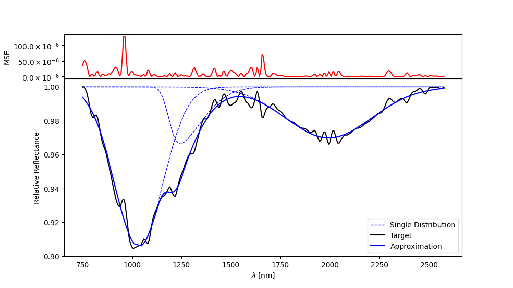
Fit diagnostics

The following methods evaluate and visualize the global fit, the local contribution of each band and the residuals.

residuals = SA.mse() # Mean square error per wavelength

SA.global_fit() # Global fit and residuals

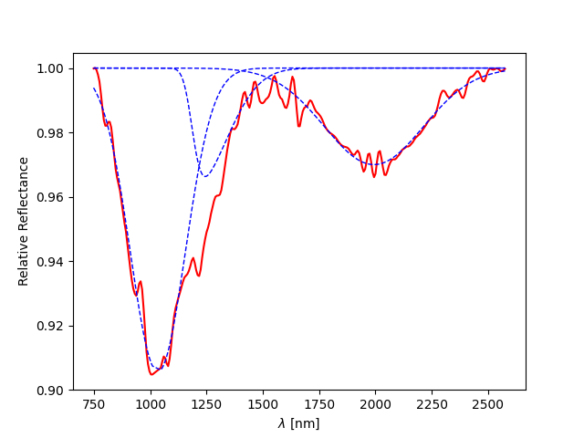
single_bands = SA.local_fit() # Single fitted distributions

all_bands = SA.both_fit() # Global fit, local bands and residuals

The outputs should then look similar to the following: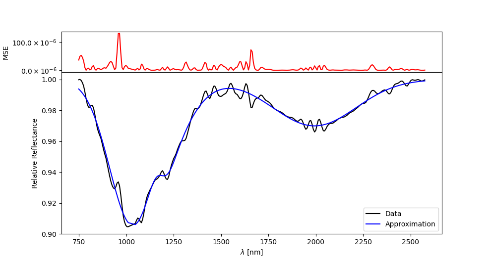

Animation of the gradient-descent fitting

The fitting history can also be animated. Set save=True to write the animation as a GIF.

SA.create_animation(losses , gaussian_sums , SA.final , n_wav ,
 frame_step = 20 ,
 FPS = 15 ,
 save = False ,
 path = 'FRT00009b5a/' ,
 name = 'mgm_gradient_descent') # Animation of the fitting process