Notebook replicating a typical hyperspectral datacube analysis done using pyfresco
[1]:
import pyfresco
Data import
In the following code cell we define the paths pointing to the img and header files of the proper hyperspectral datacube and of the summary parameters datacube. These two datacubes are the ones needed by pyFRESCO to work properly.
[2]:
path_if_mtrdr = "FRT00009b5a/frt00009b5a_07_if165j_mtr3.img" # Path to the proper hyperspectral datacube
head_if_mtrdr = "FRT00009b5a/frt00009b5a_07_if165j_mtr3.hdr" # Path to the header of the proper hyperspectral datacube

path_sr_mtrdr = "FRT00009b5a/frt00009b5a_07_sr165j_mtr3.img" # Path to the summary parameters datacube
head_sr_mtrdr = "FRT00009b5a/frt00009b5a_07_sr165j_mtr3.hdr" # Path to the header of the summary parameters datacube

img , img_sr , wavelength , sr_names = pyfresco.open_raw(path_if_mtrdr , head_if_mtrdr , path_sr_mtrdr , head_sr_mtrdr)  # Open the two datacubes

Nbands = len(wavelength)
print(sr_names)
['R770', 'RBR', 'BD530_2', 'SH600_2', 'SH770', 'BD640_2', 'BD860_2', 'BD920_2', 'RPEAK1', 'BDI1000VIS', 'R440', 'IRR1', 'BDI1000IR', 'OLINDEX3', 'R1330', 'BD1300', 'LCPINDEX2', 'HCPINDEX2', 'VAR', 'ISLOPE1', 'BD1400', 'BD1435', 'BD1500_2', 'ICER1_2', 'BD1750_2', 'BD1900_2', 'BD1900R2', 'BDI2000', 'BD2100_2', 'BD2165', 'BD2190', 'MIN2200', 'BD2210_2', 'D2200', 'BD2230', 'BD2250', 'MIN2250', 'BD2265', 'BD2290', 'D2300', 'BD2355', 'SINDEX2', 'ICER2_2', 'MIN2295_2480', 'MIN2345_2537', 'BD2500_2', 'BD3000', 'BD3100', 'BD3200', 'BD3400_2', 'CINDEX2', 'BD2600', 'IRR2', 'IRR3', 'R530', 'R600', 'R1080', 'R1506', 'R2529', 'R3920']
Creation of the false color RGB map
In the two following code cells we use pyFRESCO to create the false color and phyllosilicates RGB maps with methodology defined in Viviano-Beck et al., 2014.
[3]:
FAL = pyfresco.RGBImageManipulator(img, img_sr, 'FAL', 0, 0, 0, wavelength) # Define the object FAL

FALmap, selected_stretch = FAL.RGBmapmake(FALSE = FAL, bi = 100, clip = True, cumhist = False,
                                          preset_true_colors = False, use_false_color = False)  # Effective creation of the false color RGB map

FAL.savemap('FAL' , folder = 'FRT00009b5a' , extension = '.tif' , show = True) # saving of the RGB map in a given folder, both in txt and tif files

print('Red channel limits = ', '[', selected_stretch[0] , ',' , selected_stretch[3] , ']')
print('Green channel limits = ', '[', selected_stretch[1] , ',' , selected_stretch[4] , ']')
print('Blue channel limits = ', '[', selected_stretch[2] , ',' , selected_stretch[5] , ']')
[58, 57, 56] ['R2529', 'R1506', 'R1080']
[58, 57, 56] ['R2529', 'R1506', 'R1080']
[58, 57, 56] ['R2529', 'R1506', 'R1080']
Red channel limits =  [ 0.145 , 0.3 ]
Green channel limits =  [ 0.16 , 0.3 ]
Blue channel limits =  [ 0.15 , 0.28 ]
The output of the above cell should look like this: 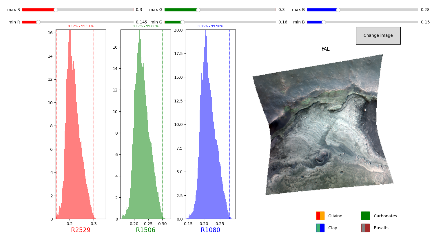
[6]:
PHY = pyfresco.RGBImageManipulator(img, img_sr, 'PHY', 0, 0, 0, wavelength) # Definition of the object PHY

phy, selected_stretch = PHY.RGBmapmake(FALSE = FALmap, bi = 500,            # Effective creation of the phyllosilicate RGB map
                                           clip = True, cumhist = False,
                                           preset_true_colors = False,
                                           use_false_color = True,
                                           R_min_in=[0,0.3] , R_max_in=[0,0.3] ,
                                           G_min_in=[0,0.03] , G_max_in=[0,0.03] ,
                                           B_min_in=[0,0.03] , B_max_in=[0,0.03] ,
                                           slider_step=0.0005)

PHY.savemap('PHY' , folder = 'FRT00009b5a' , extension = '.tif' , show = True) # Saving of the RGB map ina  given folder as in the cell above

print('Red channel limits = ', '[', selected_stretch[0] , ',' , selected_stretch[3] , ']')
print('Green channel limits = ', '[', selected_stretch[1] , ',' , selected_stretch[4] , ']')
print('Blue channel limits = ', '[', selected_stretch[2] , ',' , selected_stretch[5] , ']')
[39, 33, 26] ['D2300', 'D2200', 'BD1900R2']
[39, 33, 26] ['D2300', 'D2200', 'BD1900R2']
Red channel limits =  [ 0 , 0.0105 ]
Green channel limits =  [ 0 , 0.008 ]
Blue channel limits =  [ 0.005 , 0.027 ]
The output of the above cell should look like this: 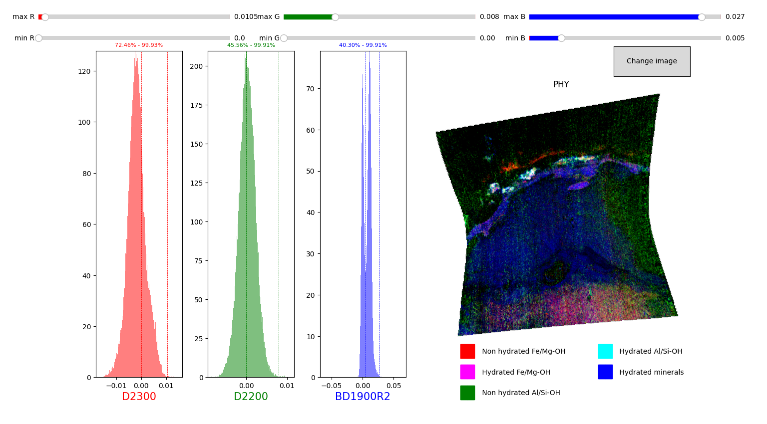
Extraction of spectra from the datacube
In the following cells we extract a spectrum from the hyperspectral datacube using the phyllosilicate RGB map as a guideline.
The spectrum will be the mean spectrum of a set of spectra inside a Region of Interest (ROI), manually selected by drawing a polygon on the phyllosilicate RGB map.
[7]:
SE = pyfresco.SpectraExtract(img , Nbands , wavelength , 750 , 2600) # Definition of the object for spectral extraction
hyd = SE.upload_map('PHY' , folder = 'FRT00009b5a')                  # Upload an RGB map for the ROI selection
[8]:
polygon_spectra , L , mask = SE.polygon_spectra(save_pixel = True ,  # Select polygonal ROI on the RGB map
                                                folder = 'FRT00009b5a' ,
                                                name = 'phy_ROI_coordinates')
polygon_spectrum , polygon_error = SE.final_spectra() # Compute mean and standard deviation spectrum of the ROI and plot it
Number of points inside the drewn polygon: 672
The outputs of the above cell should something like the following images:
Selection of the ROI by polygon: 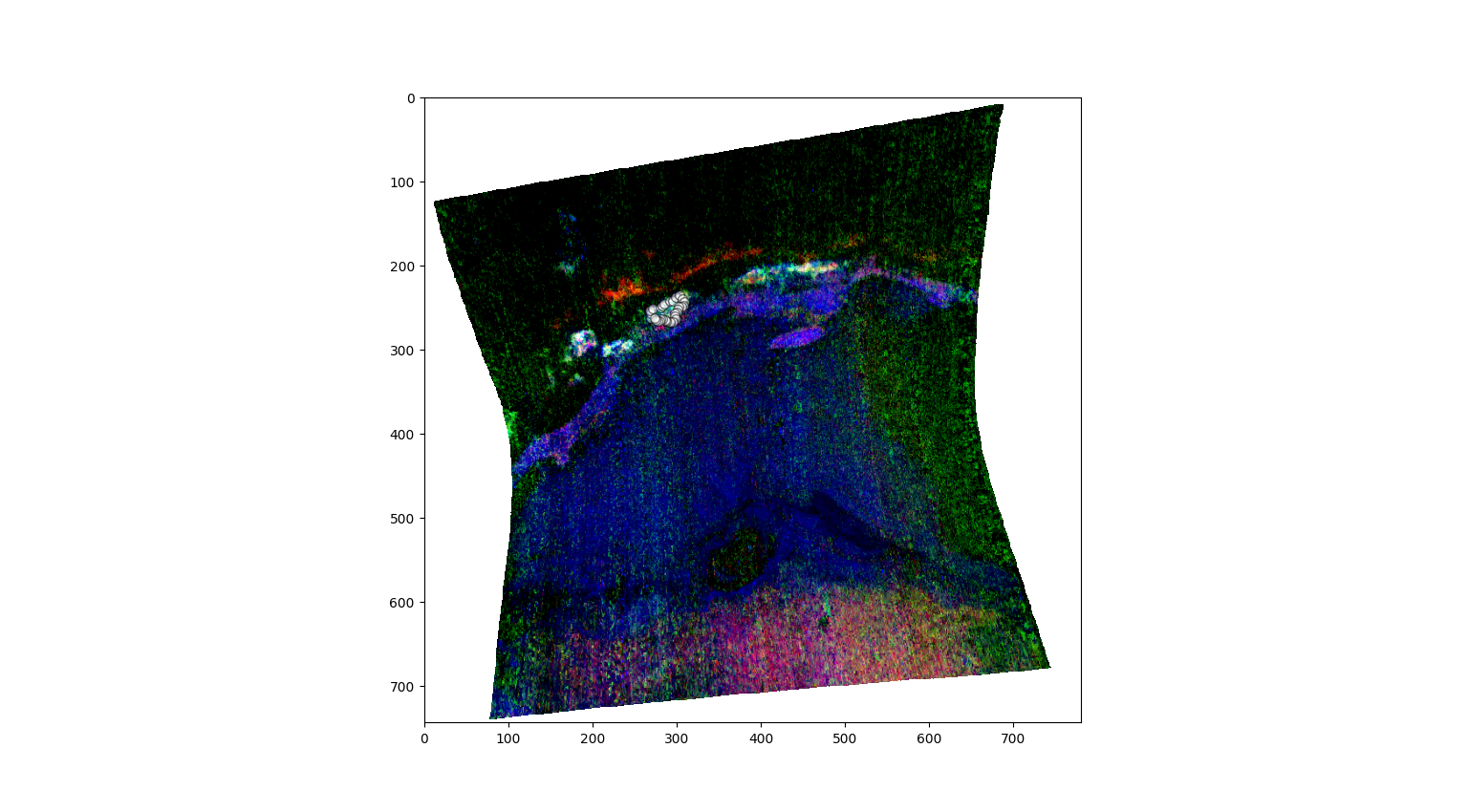
Resulting mean spectrum with stadard deviation: 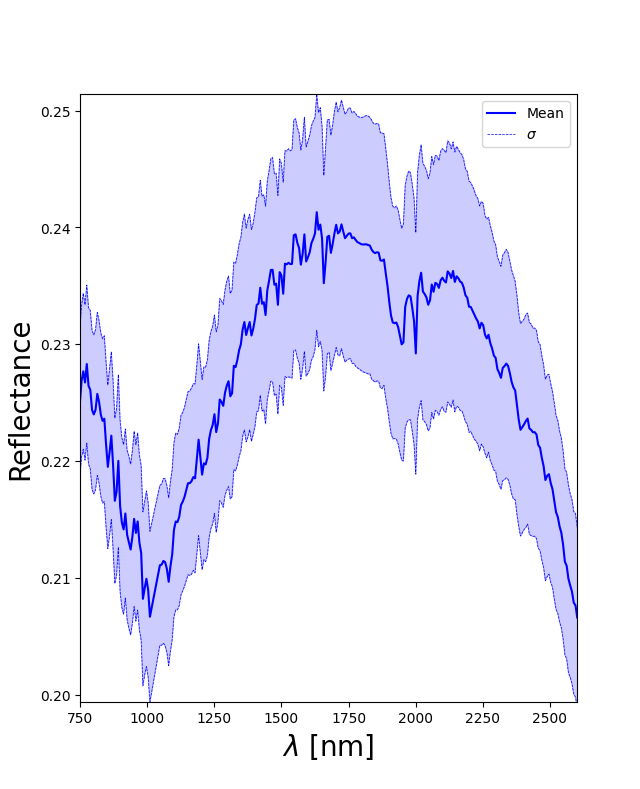
Normalization of target ROI spectrum
PyFRESCO offers various ways for the normalization of the spectrum. Following we use a ‘classically’ used method that we can call ‘Neutral Polygon Method’, in which a median spectrum from a dark ROI is selected to then perform the following operation to obtain a normalized (or ratioed) spectrum:
The further propagated error can be obtained either by classic error propagation or via a bootstrap method.
[9]:
SN = pyfresco.SpectraNorm(hyd , Nbands , img , img_sr , wavelength , # Definition of the object for spectral normalization
                 polygon_spectrum , polygon_error , polygon_spectra ,
                 750 , 2600)
[10]:
n_polygon_spectra , n_polygon , n_polygon_err , Ln , mask = SN.neutral_polygon_spectra() # Extraction of a polygon

print(polygon_spectra.shape , n_polygon_spectra.shape)

SN.plot_together()  # Plot of target and neutral spectra
normpoly , errorpoly = SN.bootstrapnorm(convexhull = False , N = 5000) # Computation of the normalized spectrum with bootstrap error
SN.normplot() # Plot fo the normalized spectrum

polynorm , polyerr = SN.norm_spectra() # Computation of the classically normalized spectrum
SN.normplot() # Plot of the normalized spectrum
Number of points inside the drewn polygon:  1450
(672, 489) (1450, 489)
0.7220216606498195 % of the errors, set to zero for simplicity, are in reality NaN values.
The outputs of the above cell should be something like:
Selection of the neutral ROI with a polygon: 
Target ROI mean spectrum and neutral ROI median spectrum: 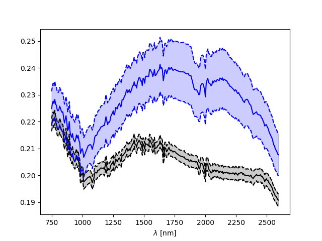
Resulting normalized spectrum with bootstrap derived error: 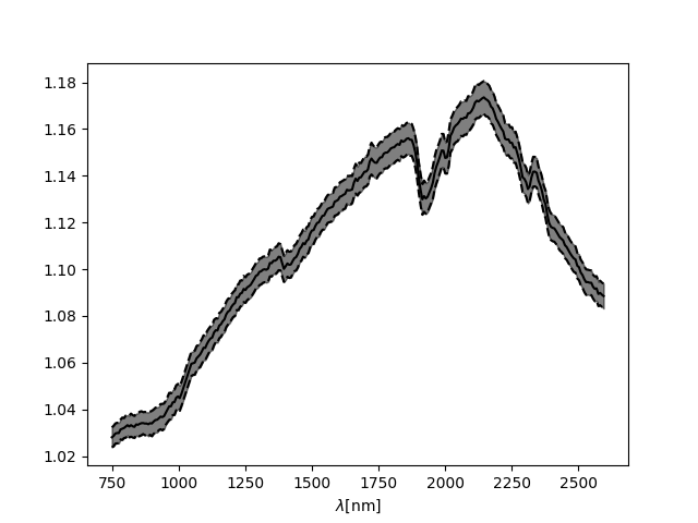
Resulting normalized spectrum with classically derived error: 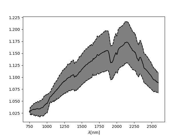
Analysis of the normalized spectrum
PyFRESCO offers various ways to ntaively analyze the normalized spectrum. Following, we use a comparison method that is based on the comparison of the absorption band positions with other, validated spectra taken from the MICA files (Viviano-Beck et al., 2015).
The comparison can be done in three ways, from less complete to more complete ones, of which the last one offers also the possibility of automatically inferring line positions given a MICA files spectrum to compare.
[11]:
SA = pyfresco.SpectraAnalysis(normpoly , errorpoly ,  # Definition of the object for spectral analysis
                     m_spec = polygon_spectrum , err_spec = polygon_error ,
                     n_spectra = n_polygon , n_err = n_polygon_err , wavelength = wavelength ,
                     MIN = 750 , MAX = 2600 , folder = None)

SA.dataset_interaction('Mg Smectite' , use = 'Both') # Displaying details of our compositional guess
C:\Users\mbaro\miniconda3\envs\pyfresco\lib\site-packages\pyfresco\SpectraAnalysis.py:257: ParserWarning: Falling back to the 'python' engine because the 'c' engine does not support sep=None with delim_whitespace=False; you can avoid this warning by specifying engine='python'.
  spectra_info = pd.read_csv('spectra_MICA_LAB_info.csv' , sep = None ,
[11]:
| Mineral Name | Mineral Type | txt name CRISM | txt name LAB | CRISM spectra cube | Lab. Mineral | Type of Lab. From MICA | MICA Lab.Code | Type of Lab. From website | Notable Absorptions CRISM [nm] | Notable Absorptions LAB [nm] | Sample Grain Size [mum] | |
|---|---|---|---|---|---|---|---|---|---|---|---|---|
| 13 | Mg Smectite | Phyllosilicate | crism_spec_mg_smectite.txt | mg_smectite_LAB.txt | FRT00009365 | Saponite | RELAB | LASA58 | GEO | [1410 , 1920 , 2310 , 2390] | [1390 , 1910 , 2320 , 2390] | max 4 |
[12]:
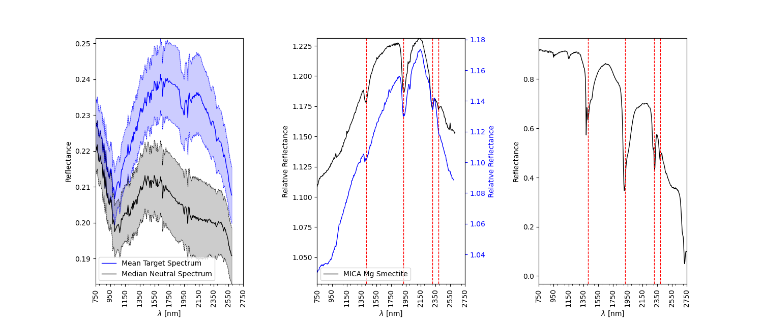
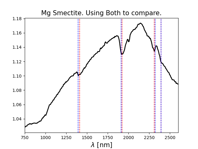
SA.simple_compare('Mg Smectite', use = 'Both') # Plot of the normalized spectrum with superimposed tabulated and validated absorption lines
The result of the above cell will be something like:
[13]:
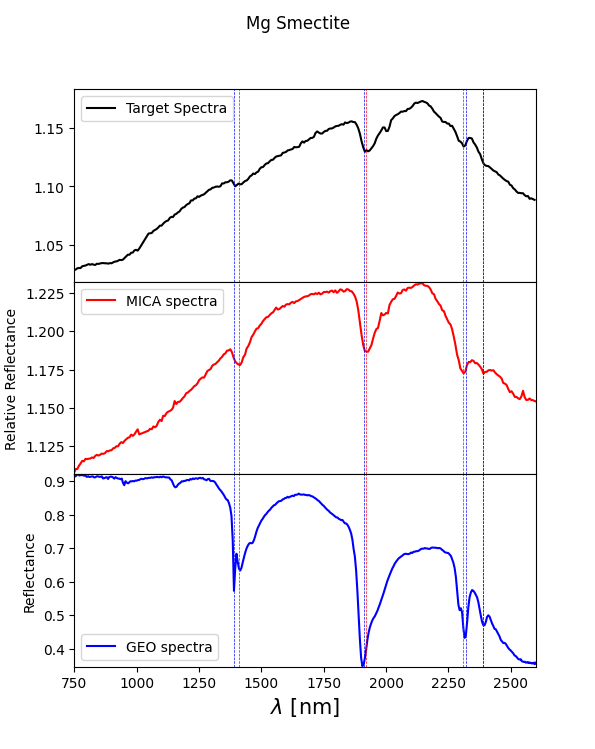
SA.compare_spectra('Mg Smectite' , use = 'Both') # Plot of the normalized spectrum with superimposed tabulated and validated absorption lines along
                                                 # with the CRISM and laboratory spectra from the MICA files
The result of the above cell will be something like:
[14]:
absoC , absoL , diffC , diffL , CRISM_abs , LAB_abs = SA.compare_lines('Mg Smectite' , ran = 5 , s = 1 , t = 1) # Automatical inferring
                                                                                                                # of absorption line positions

print('CRISM derived absorption(s) = ' , absoC)
print('CRISM derived absorption(s) difference = ' , diffC)
print('LAB derived absorption(s) =. ' , absoL)
print('LAB derived absorption(s) difference = ' , diffL)
CRISM derived absorption(s) =  [np.float64(1414.59), np.float64(1914.87), np.float64(2311.18), np.float64(2390.58)]
CRISM derived absorption(s) difference =  [np.float64(4.589999999999918), np.float64(5.130000000000109), np.float64(1.1799999999998363), np.float64(0.5799999999999272)]
LAB derived absorption(s) =.  [np.float64(1414.59), np.float64(1914.87), np.float64(2311.18), np.float64(2390.58)]
LAB derived absorption(s) difference =  [np.float64(24.589999999999918), np.float64(4.869999999999891), np.float64(8.820000000000164), np.float64(0.5799999999999272)]
[15]:
SA.compare2(0 , n_polygon , n_polygon_err , normpoly , 'Mg Smectite') # Plot of the comaprison using the inferred lines
C:\Users\mbaro\miniconda3\envs\pyfresco\lib\site-packages\pyfresco\SpectraAnalysis.py:699: ParserWarning: Falling back to the 'python' engine because the 'c' engine does not support sep=None with delim_whitespace=False; you can avoid this warning by specifying engine='python'.
  spectra_info = pd.read_csv('spectra_MICA_LAB_info.csv' , sep = None ,
The result of the above cells will be something like: