Notebook showing the MaficAnalysis method implemented in pyFRESCO
[1]:
import pyfresco
Data import
In the following code cell we define the paths pointing to the img and header files of the proper hyperspectral datacube and of the summary parameters datacube. These two datacubes are the ones needed by pyFRESCO to work properly.
[2]:
path_if_mtrdr = "FRT00009b5a/frt00009b5a_07_if165j_mtr3.img" # Path to the proper hyperspectral datacube
head_if_mtrdr = "FRT00009b5a/frt00009b5a_07_if165j_mtr3.hdr" # Path to the header of the proper hyperspectral datacube

path_sr_mtrdr = "FRT00009b5a/frt00009b5a_07_sr165j_mtr3.img" # Path to the summary parameters datacube
head_sr_mtrdr = "FRT00009b5a/frt00009b5a_07_sr165j_mtr3.hdr" # Path to the header of the summary parameters datacube

img , img_sr , wavelength , sr_names = pyfresco.open_raw(path_if_mtrdr , head_if_mtrdr , path_sr_mtrdr , head_sr_mtrdr) # Open the two datacubes

Nbands = len(wavelength)
print(sr_names)
['R770', 'RBR', 'BD530_2', 'SH600_2', 'SH770', 'BD640_2', 'BD860_2', 'BD920_2', 'RPEAK1', 'BDI1000VIS', 'R440', 'IRR1', 'BDI1000IR', 'OLINDEX3', 'R1330', 'BD1300', 'LCPINDEX2', 'HCPINDEX2', 'VAR', 'ISLOPE1', 'BD1400', 'BD1435', 'BD1500_2', 'ICER1_2', 'BD1750_2', 'BD1900_2', 'BD1900R2', 'BDI2000', 'BD2100_2', 'BD2165', 'BD2190', 'MIN2200', 'BD2210_2', 'D2200', 'BD2230', 'BD2250', 'MIN2250', 'BD2265', 'BD2290', 'D2300', 'BD2355', 'SINDEX2', 'ICER2_2', 'MIN2295_2480', 'MIN2345_2537', 'BD2500_2', 'BD3000', 'BD3100', 'BD3200', 'BD3400_2', 'CINDEX2', 'BD2600', 'IRR2', 'IRR3', 'R530', 'R600', 'R1080', 'R1506', 'R2529', 'R3920']
Target extraction and normalization
The mafic analysis works on a spectrum. Here we reproduce a compact extraction plus normalization workflow to create the input spectrum. For a real analysis, select the target and neutral ROIs on mafic-rich and spectrally neutral areas respectively.
[3]:
SE = pyfresco.SpectraExtract(img , Nbands , wavelength , 750 , 2600) # Definition of the object for spectral extraction

RGB = SE.upload_map('MAF' , folder = 'FRT00009b5a/') # Upload an RGB map for the ROI selection
[4]:
target_spectra , L_target , target_mask = SE.polygon_spectra(save_pixel = True ,
folder = 'FRT00009b5a' ,
name = 'mafic_target_coordinates') # Select the target ROI
target_spectrum , target_error = SE.final_spectra(mean = True , c = 'blue') # Target mean spectrum
SN = pyfresco.SpectraNorm(RGB , Nbands , img , img_sr , wavelength ,
target_spectrum , target_error , target_spectra ,
750 , 2600)
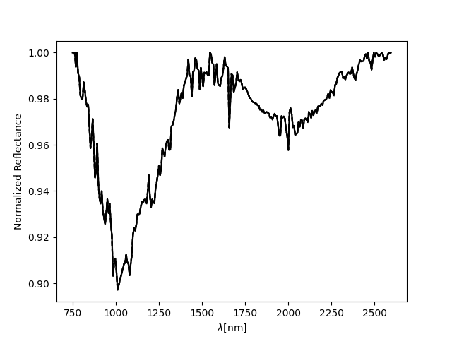
neutral_spectra , neutral_spectrum , hull_error = SN.neutral_convex_hull() # Select the neutral ROI
mafic_norm , mafic_norm_error = SN.norm_spectra(convex_hull = True) # Normalized mafic spectrum
SN.normplot()
Number of points inside the drewn polygon:  262
100.0 % of the errors, set to zero for simplicity, are in reality NaN values.
The output of the above cell should look like this: 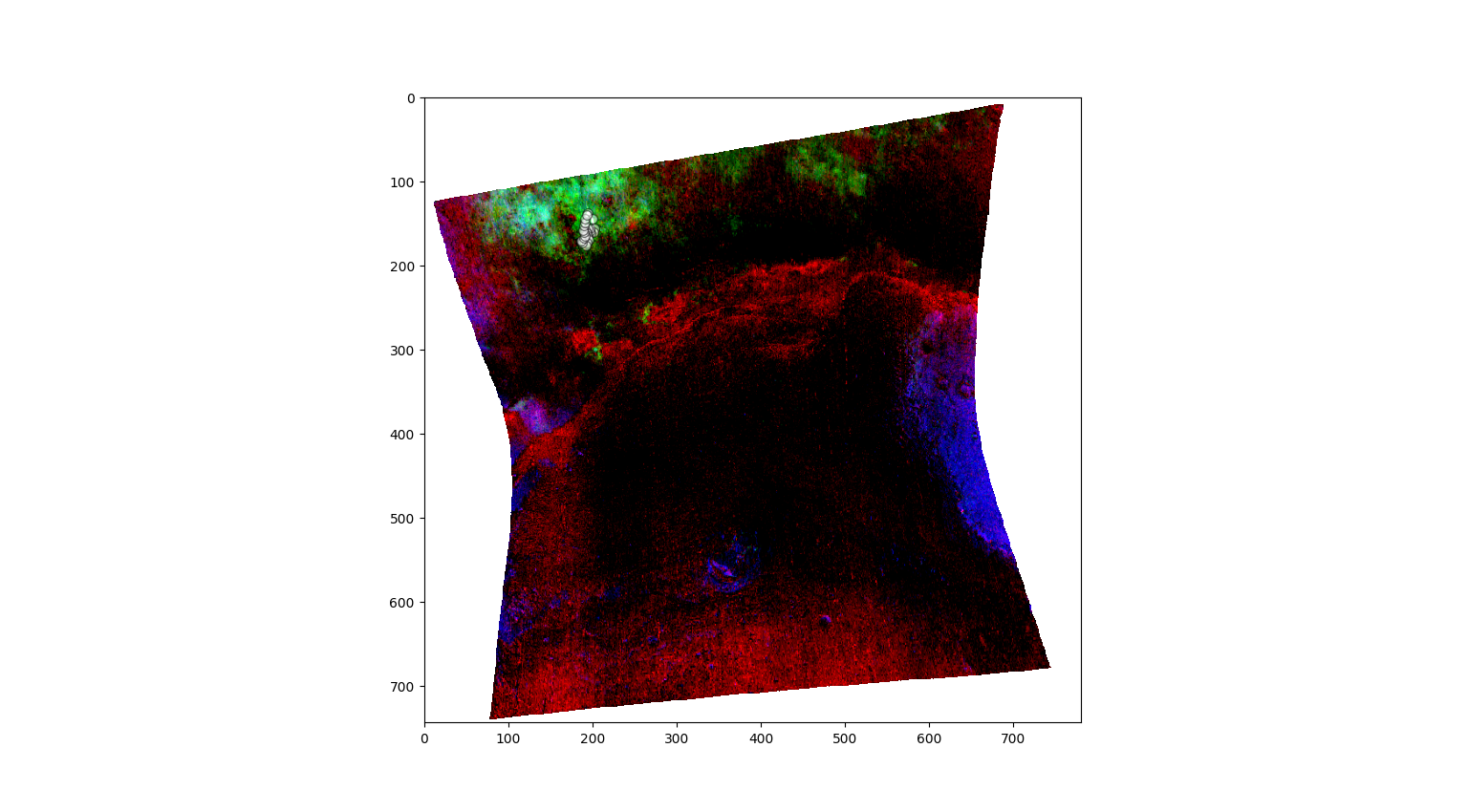
Definition of the MaficAnalysis object
The object takes the normalized spectrum, the wavelength array and the spectral interval used for the analysis.
[5]:
MA = pyfresco.MaficAnalysis(mafic_norm , wavelength , 750 , 2600 ,
 fsize = 15 ,
 pre_normed = True) # Definition of the object for mafic analysis
Band-parameter extraction
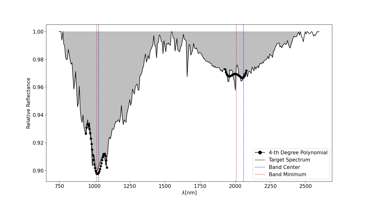
The core of the mafic analysis estimates the band extremes, band minimum, band center, band depth, band area and band asymmetry.
[6]:
parameters = MA.band_parameters(windows_nm = 75 ,
 resolution_nm = 5 ,
 plot = True ,
 tol = 10 ,
 smoothed_after_removed = False) # Compute mafic band parameters
[np.int64(0), np.int64(1), np.int64(2), np.int64(4), np.int64(117), np.int64(256), np.int64(263), np.int64(268), np.int64(274), np.int64(276)] [[  0]
 [  1]
 [  2]
 [  4]
 [117]
 [256]
 [263]
 [268]
 [274]
 [276]]
Band number  1
Band extremes =  (np.float64(774.92), np.float64(1539.48))  nm
Band minimum =  1010.18  nm
Band center =  1023.24  nm
Band depth =  0.05
Band area =  36.03  nm
Band asymmetry =  0.14  %
--------------------------------
Band number  2
Band extremes =  (np.float64(1546.06), np.float64(2456.79))  nm
Band minimum =  2000.63  nm
Band center =  2053.06  nm
Band depth =  0.01
Band area =  17.2  nm
Band asymmetry =  0.33  %
--------------------------------
The output of the above cell should look like this: