Notebook showing all the spectral normalization methods implemented in pyFRESCO

import pyfresco

Data import

In the following code cell we define the paths pointing to the img and header files of the proper hyperspectral datacube and of the summary parameters datacube. These two datacubes are the ones needed by pyFRESCO to work properly.

path_if_mtrdr = "FRT00009b5a/frt00009b5a_07_if165j_mtr3.img" # Path to the proper hyperspectral datacube
head_if_mtrdr = "FRT00009b5a/frt00009b5a_07_if165j_mtr3.hdr" # Path to the header of the proper hyperspectral datacube

path_sr_mtrdr = "FRT00009b5a/frt00009b5a_07_sr165j_mtr3.img" # Path to the summary parameters datacube
head_sr_mtrdr = "FRT00009b5a/frt00009b5a_07_sr165j_mtr3.hdr" # Path to the header of the summary parameters datacube

img , img_sr , wavelength , sr_names = pyfresco.open_raw(path_if_mtrdr , head_if_mtrdr , path_sr_mtrdr , head_sr_mtrdr) # Open the two datacubes

Nbands = len(wavelength)
print(sr_names)

['R770', 'RBR', 'BD530_2', 'SH600_2', 'SH770', 'BD640_2', 'BD860_2', 'BD920_2', 'RPEAK1', 'BDI1000VIS', 'R440', 'IRR1', 'BDI1000IR', 'OLINDEX3', 'R1330', 'BD1300', 'LCPINDEX2', 'HCPINDEX2', 'VAR', 'ISLOPE1', 'BD1400', 'BD1435', 'BD1500_2', 'ICER1_2', 'BD1750_2', 'BD1900_2', 'BD1900R2', 'BDI2000', 'BD2100_2', 'BD2165', 'BD2190', 'MIN2200', 'BD2210_2', 'D2200', 'BD2230', 'BD2250', 'MIN2250', 'BD2265', 'BD2290', 'D2300', 'BD2355', 'SINDEX2', 'ICER2_2', 'MIN2295_2480', 'MIN2345_2537', 'BD2500_2', 'BD3000', 'BD3100', 'BD3200', 'BD3400_2', 'CINDEX2', 'BD2600', 'IRR2', 'IRR3', 'R530', 'R600', 'R1080', 'R1506', 'R2529', 'R3920']

Target spectrum extraction

Before applying any normalization method we need a target ROI spectrum. Here we repeat the polygon extraction used in the first and second tutorial notebooks.

SE = pyfresco.SpectraExtract(img , Nbands , wavelength , 750 , 2600) # Definition of the object for spectral extraction

RGB = SE.upload_map('PHY' , folder = 'FRT00009b5a') # Upload an RGB map for the ROI selection

polygon_spectra , L , mask = SE.polygon_spectra(save_pixel = True ,
 folder = 'FRT00009b5a' ,
 name = 'target_polygon_coordinates') # Select the target ROI

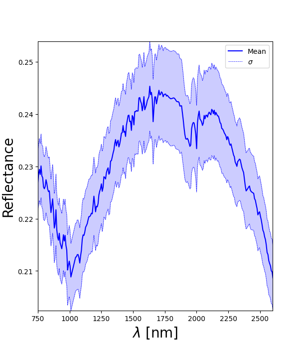
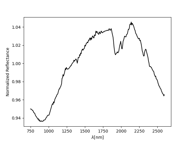
polygon_spectrum , polygon_error = SE.final_spectra(mean = True , c = 'blue') # Mean and standard deviation target spectrum

Number of points inside the drewn polygon:  297

The output of the above cell should look like this: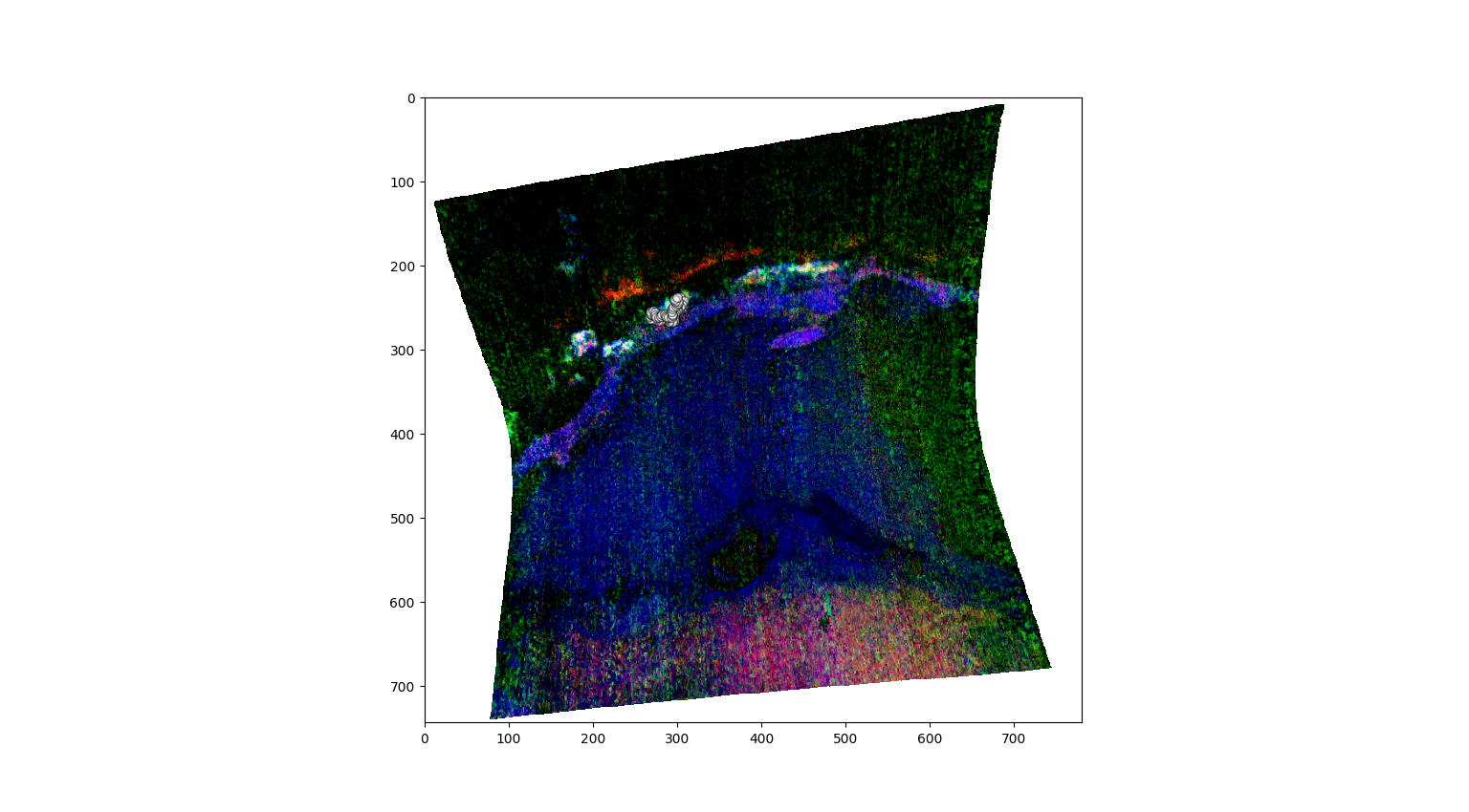

Definition of the normalization object

The same SpectraNorm object can be reused to test different neutral-spectrum choices. Each method overwrites the currently stored neutral spectrum, so the normalization is computed immediately after each neutral selection.

SN = pyfresco.SpectraNorm(RGB , Nbands , img , img_sr , wavelength , # Definition of the object for spectral normalization
 polygon_spectrum , polygon_error , polygon_spectra ,
 750 , 2600)

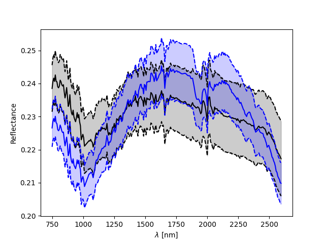
Neutral Polygon Method

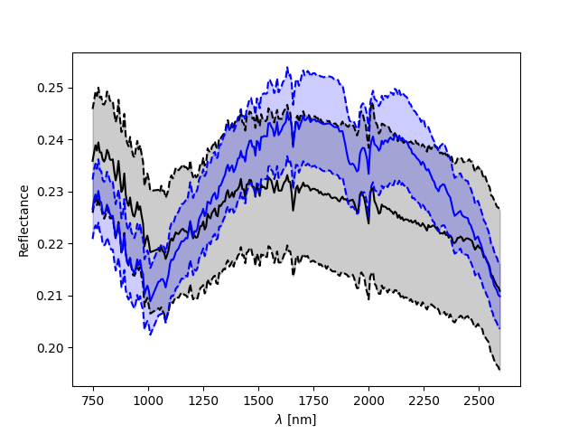
The first normalization method uses a manually selected neutral polygon. The median spectrum of this neutral ROI is used as denominator for the target spectrum.

neutral_polygon_spectra , neutral_polygon , neutral_polygon_error , L_neutral , mask_neutral = SN.neutral_polygon_spectra(
 save_pixel = True ,
 folder = 'FRT00009b5a' ,
 name = 'neutral_polygon_coordinates') # Draw a neutral ROI

SN.plot_together() # Plot target and neutral spectra

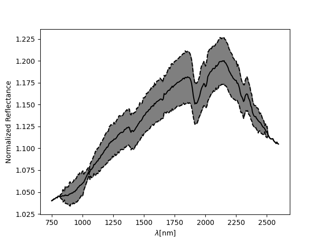
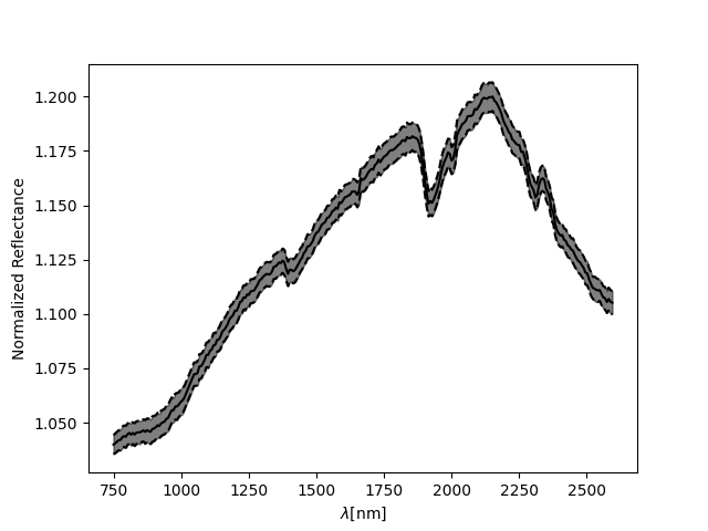
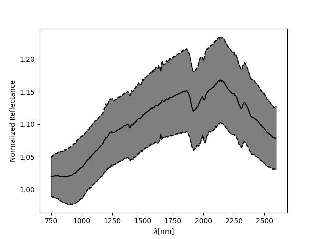
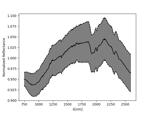
norm_polygon , error_polygon = SN.norm_spectra() # Classical ratio and propagated error
SN.normplot()

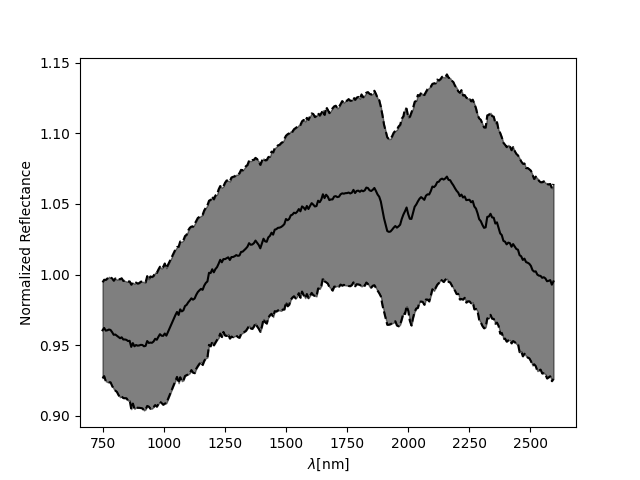
norm_polygon_boot , error_polygon_boot = SN.bootstrapnorm(convexhull = False , N = 5000) # Bootstrap normalization
SN.normplot()

Number of points inside the drewn polygon:  2150
9.386281588447654 % of the errors, set to zero for simplicity, are in reality NaN values.

The output of the above cell should look like this: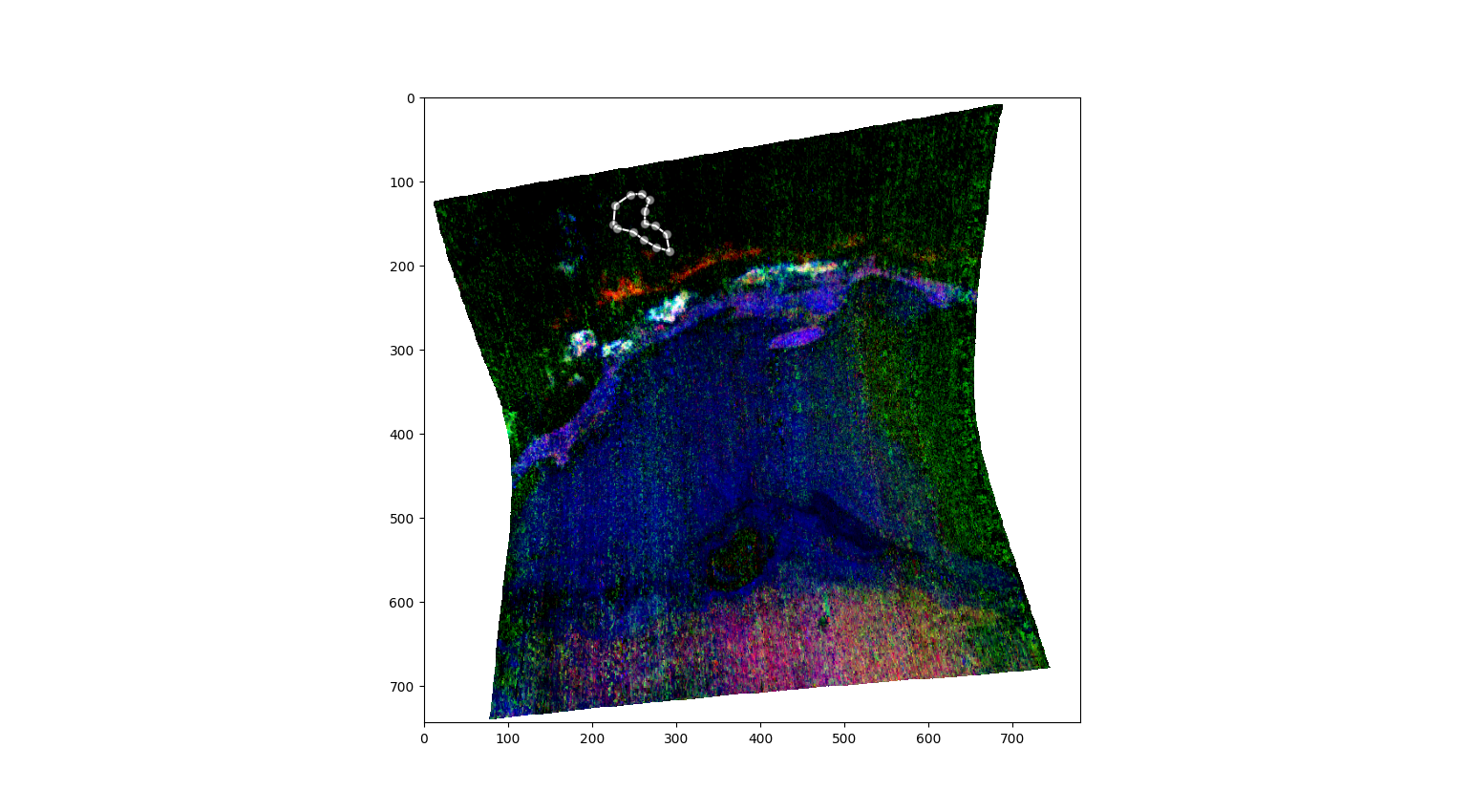

Convex Hull Method

The convex hull method uses the continuum of the target spectrum as neutral spectrum. This is useful when an external neutral ROI is not available.

neutral_hull , hull_spectrum , hull_error = SN.neutral_convex_hull(interp = 'linear') # Compute the convex hull neutral spectrum

SN.plot_together(convex_hull = True)

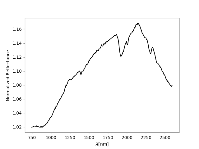
norm_hull , error_hull = SN.norm_spectra(convex_hull = True) # Normalize using the convex hull
SN.normplot(convex_hull = True)

norm_hull_boot , error_hull_boot = SN.bootstrapnorm(convexhull = True , N = 5000) # Bootstrap version
SN.normplot(convex_hull = True)

100.0 % of the errors, set to zero for simplicity, are in reality NaN values.

The output of the above cell should look like this: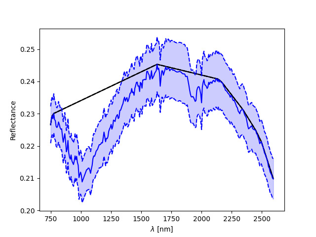

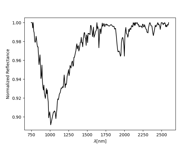
Single All-Map Method

The single all-map method searches for pixels with low values in one RGB map. Those pixels are used to build the neutral spectrum.

neutral_single , neutral_single_median , neutral_single_mad , x_single , y_single = SN.neutral_all_map_single(threshold = 0) # Search low-valued pixels in the current RGB map

SN.plot_together()

norm_single , error_single = SN.norm_spectra()
SN.normplot()

norm_single_boot , error_single_boot = SN.bootstrapnorm(convexhull = False , N = 5000) # Bootstrap version
SN.normplot(convex_hull = True)

0.0 % of the errors, set to zero for simplicity, are in reality NaN values.

The output of the above cell should look like this:

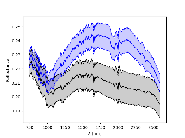
Multiple All-Map Method

The multiple all-map method repeats the same low-value pixel search on several RGB maps. Only pixels satisfying the requested overlap condition are retained.

RGBs_names = ['HYD' , 'PHY' , 'MAF'] # RGB maps previously saved with RGBImageManipulator.savemap()
RGB_path = 'FRT00009b5a/'

neutral_multiple , neutral_multiple_median , neutral_multiple_mad , superimposed , zero_map , xx , yy = SN.neutral_all_map_multiple(
 RGBs_names = RGBs_names ,
 RGB_path = RGB_path ,
 p = len(RGBs_names) ,
 threshold = 0 ,
 names = RGBs_names)

SN.plot_together()

norm_multiple , error_multiple = SN.norm_spectra()
SN.normplot()

norm_multiple_boot , error_multiple_boot = SN.bootstrapnorm(convexhull = False , N = 5000) # Bootstrap version
SN.normplot(convex_hull = True)

0.0 % of the errors, set to zero for simplicity, are in reality NaN values.

The output of the above cell should look like this:

Mineral Mask Method

The mineral mask method uses spectral-parameter thresholds to select the neutral pixels. Reflectance parameters are treated differently from band-depth parameters.

band_names = ['R770' , 'BDI1000IR' , 'OLINDEX3' , 'BD1300' , 'LCPINDEX2' , 'HCPINDEX2',
             'D2200' , 'BD2290' , 'D2300' , 'BD2500_2' , 'SINDEX2' , 'BD1900_2']
band_values = [0.23,0.035,0.09,0,0,0,0.001,0.001,0.001,0,0.0045,0.012]

neutral_mask , neutral_mask_median , neutral_mask_mad = SN.mineral_mask(
 b = 500 ,
 band_n = band_names ,
 band_v = band_values)

SN.plot_together()

norm_mask , error_mask = SN.norm_spectra()
SN.normplot()

norm_mineralmask_boot , error_mineralmask_boot = SN.bootstrapnorm(convexhull = False , N = 5000) # Bootstrap version
SN.normplot(convex_hull = True)

constraints_mask.size=581064
constraints_mask.sum()=np.int64(13961)
0.0 % of the errors, set to zero for simplicity, are in reality NaN values.

The output of the above cell should look like this: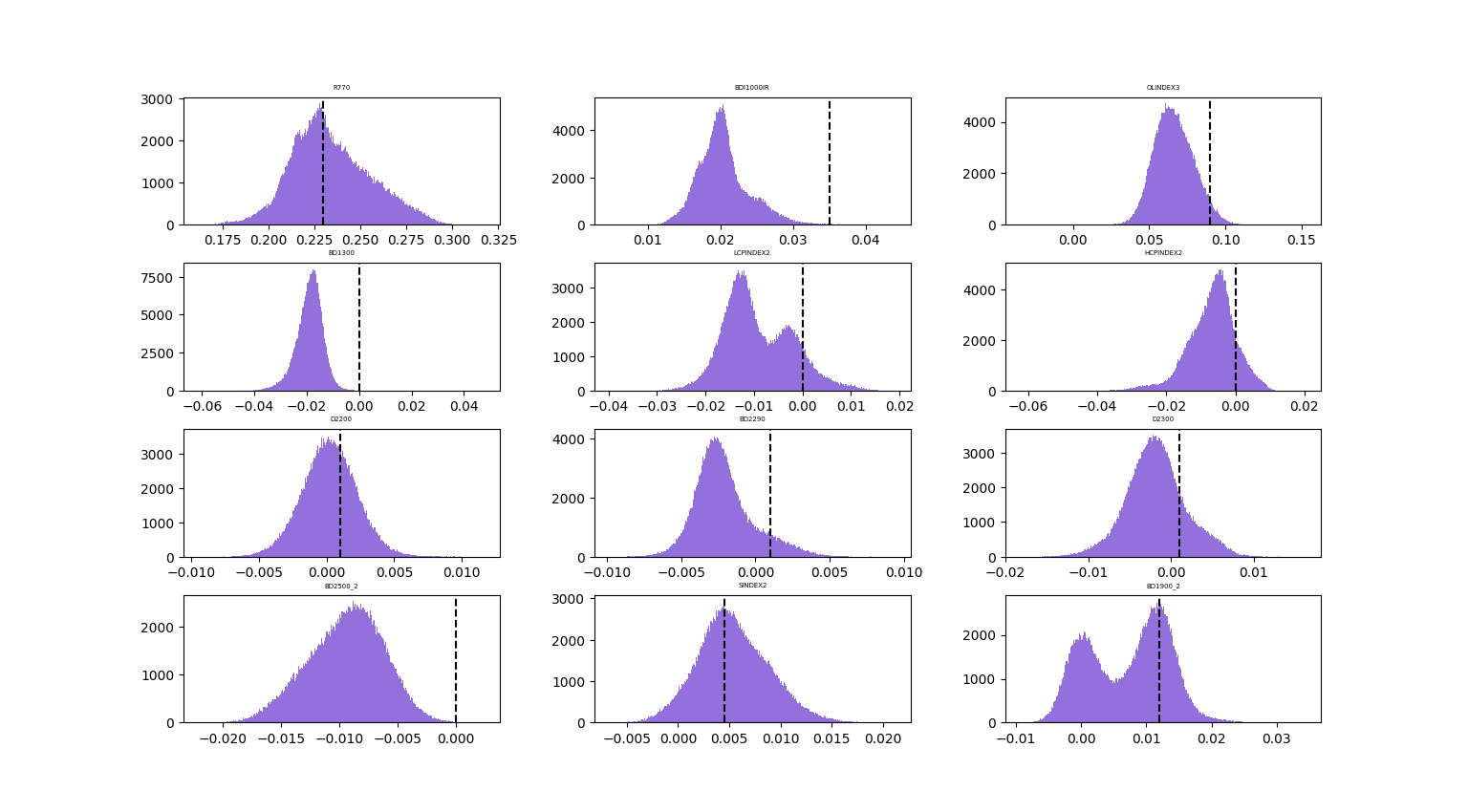

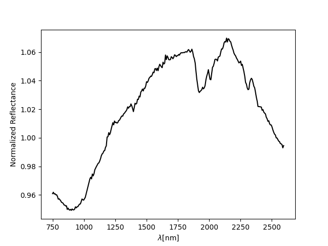
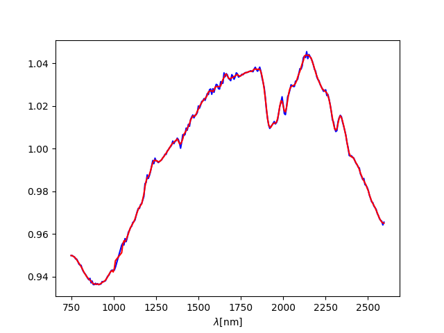
Smoothing of the normalized spectrum

After any normalization, the normalized spectrum can be smoothed with either a moving average or a Savitzky-Golay filter.

smooth_movmean = SN.moving_average(window_size = 5) # Moving average smoothing

smooth_savgol = SN.savgol(window = 7 , order = 2) # Savitzky-Golay smoothing

The output of the above cell should look like this: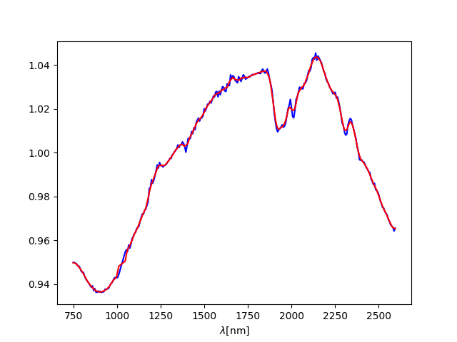

Saving normalized spectra

The normalized spectrum and associated neutral spectrum can be saved for later analysis notebooks.

SN.save_spectrum(name = 'target_polygon' ,
 folder = 'FRT00009b5a/' ,
 method = 'min' ,
 normalized = True)