Notebook showing all the spectral extraction methods implemented in pyFRESCO

import pyfresco

Data import

In the following code cell we define the paths pointing to the img and header files of the proper hyperspectral datacube and of the summary parameters datacube. These two datacubes are the ones needed by pyFRESCO to work properly.

path_if_mtrdr = "FRT00009b5a/frt00009b5a_07_if165j_mtr3.img" # Path to the proper hyperspectral datacube
head_if_mtrdr = "FRT00009b5a/frt00009b5a_07_if165j_mtr3.hdr" # Path to the header of the proper hyperspectral datacube

path_sr_mtrdr = "FRT00009b5a/frt00009b5a_07_sr165j_mtr3.img" # Path to the summary parameters datacube
head_sr_mtrdr = "FRT00009b5a/frt00009b5a_07_sr165j_mtr3.hdr" # Path to the header of the summary parameters datacube

img , img_sr , wavelength , sr_names = pyfresco.open_raw(path_if_mtrdr , head_if_mtrdr , path_sr_mtrdr , head_sr_mtrdr) # Open the two datacubes

Nbands = len(wavelength)
print(sr_names)

['R770', 'RBR', 'BD530_2', 'SH600_2', 'SH770', 'BD640_2', 'BD860_2', 'BD920_2', 'RPEAK1', 'BDI1000VIS', 'R440', 'IRR1', 'BDI1000IR', 'OLINDEX3', 'R1330', 'BD1300', 'LCPINDEX2', 'HCPINDEX2', 'VAR', 'ISLOPE1', 'BD1400', 'BD1435', 'BD1500_2', 'ICER1_2', 'BD1750_2', 'BD1900_2', 'BD1900R2', 'BDI2000', 'BD2100_2', 'BD2165', 'BD2190', 'MIN2200', 'BD2210_2', 'D2200', 'BD2230', 'BD2250', 'MIN2250', 'BD2265', 'BD2290', 'D2300', 'BD2355', 'SINDEX2', 'ICER2_2', 'MIN2295_2480', 'MIN2345_2537', 'BD2500_2', 'BD3000', 'BD3100', 'BD3200', 'BD3400_2', 'CINDEX2', 'BD2600', 'IRR2', 'IRR3', 'R530', 'R600', 'R1080', 'R1506', 'R2529', 'R3920']

Uploading the RGB map

In the following cells we upload the RGB map used as visual guide for the selections. The map is the one saved in the first tutorial notebook.

SE = pyfresco.SpectraExtract(img , Nbands , wavelength , 750 , 2600) # Definition of the object for spectral extraction

RGB = SE.upload_map('PHY' , folder = 'FRT00009b5a') # Upload an RGB map for the ROI selection

Point extraction

In this extraction method we manually select single pixels on the RGB map. The extracted spectra correspond to the clicked points and can be plotted one by one before computing the final spectrum.

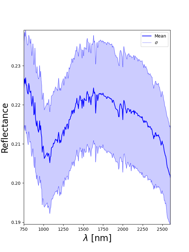
point_spectra = SE.point_spectra(N = 5) # Select 5 points on the RGB map

point_spectrum , point_error = SE.final_spectra(mean = True , c = 'blue') # Mean and standard deviation spectrum

The output of the above cell should look like this (the selected pixels are the ones with the red cross over it, remember that the last selected pixel will not have the cross!):

Square extraction

In this extraction method we select the center of a square ROI. The value of N is the side length of the square, and it must be an odd number.

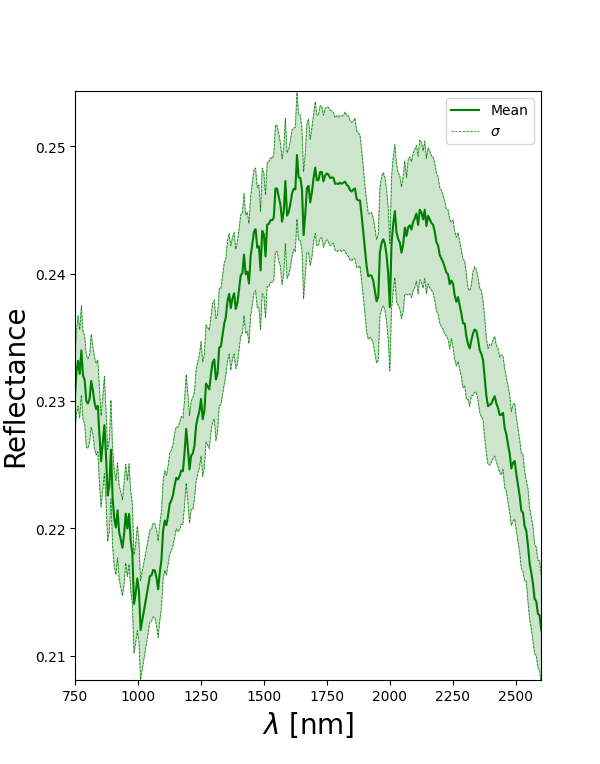
square_spectra , x_square , y_square = SE.square_spectra(N = 11 , show = True) # Select the center of an 11 x 11 pixels square

square_spectrum , square_error = SE.final_spectra(mean = True , c = 'green') # Mean and standard deviation spectrum

print('Square center = ' , x_square , y_square)

Square center =  301 247

The output of the above cell should look like this (remember that the square is selected in another image by clicking the right mouse button!):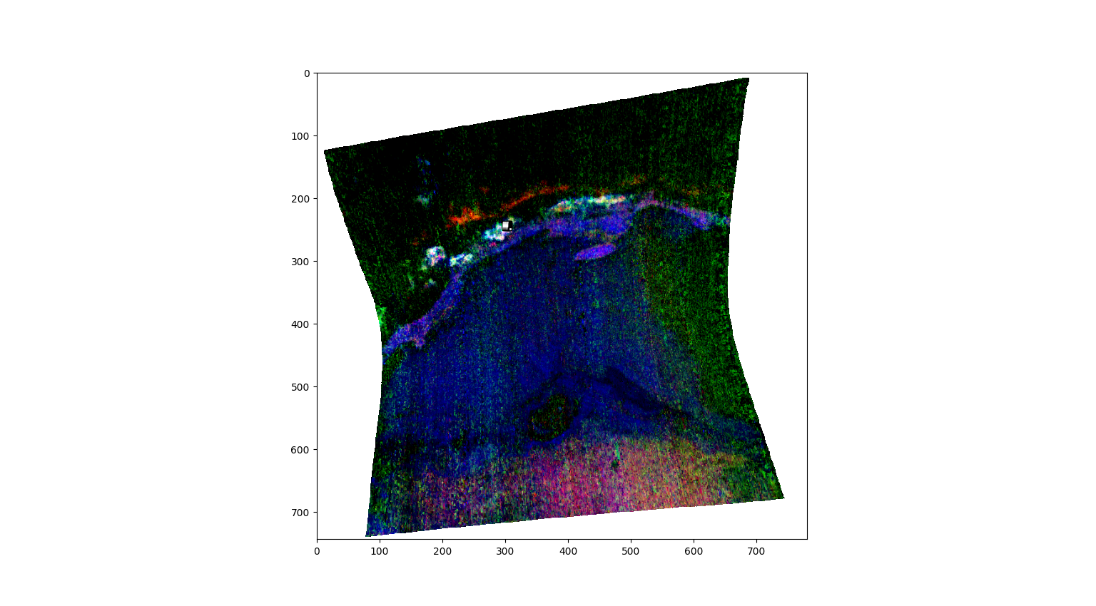

Polygon extraction

In this extraction method we draw a polygonal ROI on the RGB map. The spectra are extracted from all the pixels inside the drawn polygon.

polygon_spectra , L , mask = SE.polygon_spectra(save_pixel = True , # Select polygonal ROI on the RGB map
 folder = 'FRT00009b5a' ,
 name = 'polygon_ROI_coordinates')

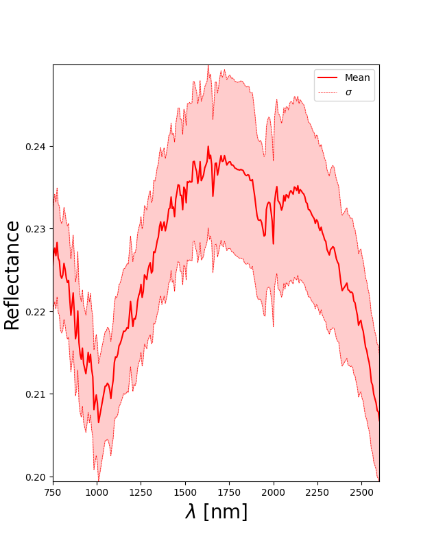
polygon_spectrum , polygon_error = SE.final_spectra(mean = True , c = 'red') # Mean and standard deviation spectrum

print('Number of polygon pixels = ' , L)

Number of points inside the drewn polygon:  796
Number of polygon pixels =  796

The output of the above cell should look like this: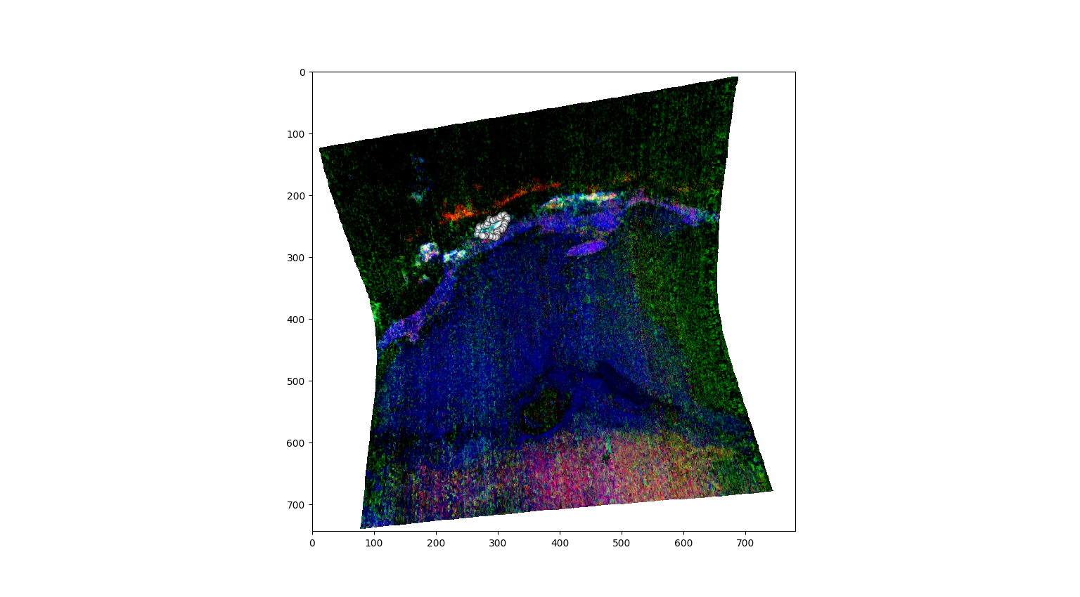

Median spectrum and MAD

The same final extraction step can be repeated using the median spectrum and the Median Absolute Deviation instead of the mean spectrum and standard deviation. This is useful when the selected ROI contains outliers.

polygon_median , polygon_mad = SE.final_spectra(mean = False , c = 'black') # Median and MAD spectrum

The output of the above cell should look like this: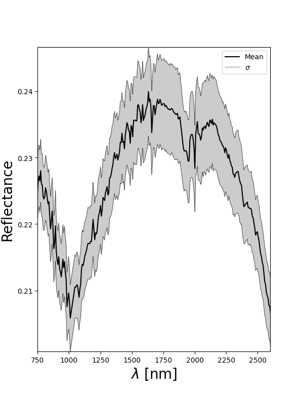

Saving the extracted spectra

The selected spectra can be saved and then reused for the other modules.

SE.save_spectra(name = 'polygon_ROI_spectra' ,
 folder = 'FRT00009b5a/' ,
 method = 'polygon') # Save the extracted spectra and the wavelength range

SE.save_spectrum(name = 'polygon_ROI_mean_spectra' ,
 folder = 'FRT00009b5a/' ,
 method = 'polygon') # Save the extracted spectra and the wavelength range